A meandering introduction to VAEs - part 4

We can find a consistent estimator by not using Jensens inequality,

\[\begin{align} \log p(x \vert \theta) &= \log \mathbb{E}_{z_i \sim p(z)} p(x \vert z, \theta) \\ &= \log \lim_{N \rightarrow \infty} \frac{1}{N} \sum_{i=1}^K p(x \vert z_i \sim p(z), \theta) \\ &= \lim_{N \rightarrow \infty} \log \frac{1}{N} \sum_{i=1}^K p(x \vert z_i \sim p(z), \theta) \,, \end{align}\]

where the last line is allowed since $\log$ is continous. This is kind of intuitive, as we take more and more samples, the term inside the log approaches $p(x \vert \theta)$, and in the limit it is $p(x \vert \theta)$, so taking the log gives us $\log p(x \vert \theta)$.

What happens when we don’t take an infinite number of samples though? We can show that it is a biased estimator by using Jensens again,

\[\begin{align} \log p(x \vert \theta) &= \log \mathbb{E}_{z_1, ..., z_N \sim p(z)} \frac{1}{N} \sum_{i=1}^N p(x \vert z_i, \theta) \\ \log p(x \vert \theta) &\geq \mathbb{E}_{z_1, ..., z_N \sim p(z)} \log \frac{1}{N} \sum_{i=1}^N p(x \vert z_i, \theta) = L_N \end{align}\]

Admittedly, this expression can be hard to understand. In the first line we’re taking an expectation over $N$ sample averages. Think of it this way: we sample a $J \times N$ matrix of $z$’s from $p(z)$, and then the inner sum is over the second dimension ($N$), and the expectation is a sum over the first dimension, where we have an infinite amount of samples $J$. This means we’re effectively taking an average with an infinite amount of samples, so we get the expectation back. Another way to think about it is that we’re summing the same infinite amount of samples just in different order. We get the second line by applying Jensens inequality.

So now we can see that the full expression is a lower bound, and the term inside the expectation is a biased but consistent estimate. We already know what happens as $N \rightarrow \infty$, then the bound becomes an equality. We can also see what happens when $N=1$, which is that we recover our previous bound, $\log p(x \vert \theta) \geq \mathbb{E}_{z_1 \sim p(z)} \log p(x \vert z_1, \theta)$, which we know didn’t work very well. It can be proven that as $N$ increases the bound becomes tighter, such that $L_k \geq L_m$ for $k \geq m$.

You can see this notebook for some code that shows what happens as $N$ increases. For now, we’ll press ahead. We can estimate the lower bound $L_N$ with $J$ outer samples and $N$ inner samples and maximizing it we’ll be maximizing an approximate lower bound on $\log p(x \vert \theta)$. Notice that now there’s both inner and outer samples. More inner samples make the bound tighter, i.e. brings us closer to $\log p(x \vert \theta)$, and more outer samples reduce the variance on the estimate of this bound. We’ve seen where $N=1$ and $J=128$ got us in the last experiment, so now we’ll try the other way so that $J=1$ and $N=128$. In short we will be maximizing the right thing estimated poorly, instead of maximizing the wrong thing, estimated accurately.

One final trick before we can start implementing. The astute reader will notice that we’re still computing in probabilities inside the sum, and not log-probabilities. However, with a little arithmetic, we can use the logsumexp trick. The logsumexp trick is a trick for computing functions of the form $f(x) = \log \sum_i e^{x_i}$, in a numerically stable way.

\[\begin{align} \log \frac{1}{N} \sum_{i=1}^N p(x \vert z_i \sim p(z), \theta) &= \log \frac{1}{N} \sum_{i=1}^N \exp{\log{p(x \vert z_i \sim p(z), \theta)}} \\ &= \text{logsumexp}_{i=1}^N \left[ \log p(x \vert z_i \sim p(z), \theta) \right]- \log N \,. \end{align}\]

Let’s code it up. The code is identical for the last model, except a single line in the loss, which I’ve highlighted.

import torch as t
import matplotlib.pyplot as plt
from torch.distributions import Normal, Bernoulli
from torchvision import datasets, transforms
import tqdm

assert t.cuda.is_available(), "requires GPU"
device = "cuda"

# Setup data

train_data = datasets.MNIST('/data/', train=True, download=True).data.reshape(-1, 28*28) # (60000, 784)
static = Bernoulli(probs=train_data/255).sample().to(device)

def train_batch(batch_size):
  idx = t.randint(static.shape[0], (batch_size,))
  return static[idx]

# Set hyper-parameters

K = 2
n_hid = 512
n_samples = 128
batch_size = 256
n_train_iters = 1_000

# Setup model
p_z = Normal(loc=t.zeros(K, device=device), scale=t.ones(K, device=device))
nn = t.nn.Sequential(
    t.nn.Linear(2, n_hid), t.nn.ELU(),
    t.nn.Linear(n_hid, n_hid), t.nn.ELU(),
    t.nn.Linear(n_hid, n_hid), t.nn.ELU(),
    t.nn.Linear(n_hid, 784),
).to(device)
nn[-1].bias.data = t.log(static.mean(dim=0)+1e-6) # just a small trick to speed up convergence
print(nn)

# Optimize the model
optim = t.optim.Adam(nn.parameters())
pbar = tqdm.tqdm(range(n_train_iters))
losses = []
for i in pbar:
  x = train_batch(batch_size) #(batch_size, 784)

  # Compute the loss
  z = p_z.sample((batch_size, n_samples)) # step 1. z ~ p(z). shape: (batch_size, n_samples, 2)
  logp = nn(z) #Step 2. shape: (batch_size, n_samples, 784)
  logpx = Bernoulli(logits=logp).log_prob(x.unsqueeze(1)).sum(dim=2) #Step 3. x ~ p(x  \vert  z, 𝜃). shape: (batch_size, n_samples) 
  # >>>>>>>>>>>>>>>>>>>>>>>>>>>>>> The line below is the only difference from the previous model! <<<<<<<<<<<<<<<<<<<<<<<<<<<<<<
  logpx = t.logsumexp(logpx, dim=1) - t.log(t.tensor(n_samples)) # (batch_size, ) 
  loss = -logpx.mean()
  
  # Take a SGD step
  optim.zero_grad()
  loss.backward()
  optim.step()

  pbar.set_description("loss: %.3f"%(loss.item()))
  losses.append(loss.item())

Sequential(
  (0): Linear(in_features=2, out_features=512, bias=True)
  (1): ELU(alpha=1.0)
  (2): Linear(in_features=512, out_features=512, bias=True)
  (3): ELU(alpha=1.0)
  (4): Linear(in_features=512, out_features=512, bias=True)
  (5): ELU(alpha=1.0)
  (6): Linear(in_features=512, out_features=784, bias=True)
)
loss: 142.500: 100% \vert ██████████ \vert  1000/1000 [02:30<00:00,  6.64it/s]

plt.plot(losses)
plt.xlabel("steps")
plt.ylabel("loss")
plt.show()

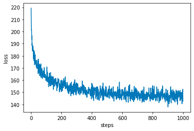
This looks much better. The loss is also much lower now. Now let’s sample from the model and see if it has learned something!

z = p_z.sample((64,))
x_samples = Bernoulli(logits=nn(z)).sample() # (64, 784)
fig, axes = plt.subplots(8, 8, dpi=100)
for i, ax in enumerate(axes.flatten()):
  ax.imshow(1-x_samples[i].detach().cpu().reshape(28, 28), interpolation="none", cmap="gray")
  ax.axis("off")
plt.show()

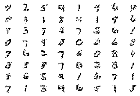
Not too shabby! There’s clearly recognizable digits in there. These are actual samples from our generative model following the recipe we set up: 1) sample from the prior $z \sim p(z)$, 2) push the $z$ values through our (now learned) network generating $784$ probabilities, 3) sample from the $784$ dimensional Bernoulli with those probabilities. Let’s also look at the average samples

p = t.sigmoid(nn(z)) # (64, 784)
fig, axes = plt.subplots(8, 8, dpi=100)
for i, ax in enumerate(axes.flatten()):
  ax.imshow(1-p[i].detach().cpu().reshape(28, 28), interpolation="none", cmap="gray")
  ax.axis("off")
plt.show()

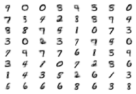
What about the loss? We get around 147, but what does that mean? By our definition of the loss, $L \approx -\log p(x \vert \theta)$, this is a (biased) estimate of the average negative log probability of a digit under our model. We can also think of it in another way. If the network outputs probability $p$ whenever a pixel is on, and $1-p$ whenever it is off, then it will have a loss of $-\log p(x \vert \theta) = -784\log p$, so inserting our approximate loss we get, $147 = -784\log p$ and solving for $p$ we get $p = \exp(-147/784)) \approx 0.83$. So, very hand-wavy, on average, the network is $83\%$ correct.

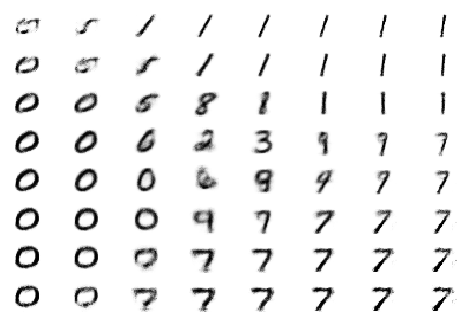
Another fun thing we can do, is to look at how the network decodes a grid of $z$ values.

z = t.stack(t.meshgrid(t.linspace(-3, 3, 8), t.linspace(-3, 3, 8)), dim=2).reshape(-1, 2).to(device) #(64, 2)
p = t.sigmoid(nn(z)) # (64, 784)
fig, axes = plt.subplots(8, 8, dpi=100)
for i, ax in enumerate(axes.flatten()):
  ax.imshow(1-p[i].detach().cpu().reshape(28, 28), interpolation="none", cmap="gray")
  ax.axis("off")
plt.show()

All in all this is a pretty good result. We set out to create a generative model of MNIST digits, and through pure sampling from the prior we managed to train a pretty decent model! We’re not at the VAE yet, but we’re getting there. The long way around.

Hosted on GitHub Pages — Theme by orderedlist