A meandering introduction to VAEs - part 3

So what can we do if we want to estimate $\log p(x \vert \theta)$? Well, we can push the log into the expectation using Jensens inequality, since log is a concave function. This turns the right hand side into a lower bound on $\log p(x \vert \theta)$.

\[\begin{align} \log p(x \vert \theta) &= \log \mathbb{E}_{z \sim p(z)} p(x \vert z, \theta) \\ &\geq \mathbb{E}_{z \sim p(z)} \log p(x \vert z, \theta) \\ \end{align}\]

If we maximize the lower bound, we’ll be “pushing up” $\log p(x \vert \theta)$ from below, so that it’s at least greater than this lower bound. Again, we can’t sample an infinite amount of samples, so we will approximate this lower bound with $N$ samples. So to be clear, we’ll be optimizing an approximate lower bound. We’ll use minibatch SGD to maximize this estimate (actually we’ll minimize the negative of this estimate, purely due to convention).

Let’s code it. This is a decent amount of code. I’ve tried to make it as simple as possible. Please make sure you understand what’s going on.

import torch as t
import matplotlib.pyplot as plt
from torch.distributions import Normal, Bernoulli
from torchvision import datasets, transforms
import tqdm

assert t.cuda.is_available(), "requires GPU"
device = "cuda"

# Setup data

train_data = datasets.MNIST('/data/', train=True, download=True).data.reshape(-1, 28*28) # (60000, 784)
static = Bernoulli(probs=train_data/255).sample().to(device)

def train_batch(batch_size):
  idx = t.randint(static.shape[0], (batch_size,))
  return static[idx]

# Set hyper-parameters

K = 2
n_hid = 512
n_samples = 128
batch_size = 256
n_train_iters = 1_000

# Setup model
p_z = Normal(loc=t.zeros(K, device=device), scale=t.ones(K, device=device))
nn = t.nn.Sequential(
    t.nn.Linear(2, n_hid), t.nn.ELU(),
    t.nn.Linear(n_hid, n_hid), t.nn.ELU(),
    t.nn.Linear(n_hid, n_hid), t.nn.ELU(),
    t.nn.Linear(n_hid, 784),
).to(device)
nn[-1].bias.data = t.log(static.mean(dim=0)+1e-6) # just a small trick to speed up convergence.
print(nn)

# Optimize the model
optim = t.optim.Adam(nn.parameters())
pbar = tqdm.tqdm(range(n_train_iters))
losses = []
for i in pbar:
  x = train_batch(batch_size) #(batch_size, 784)

  # Compute the loss
  z = p_z.sample((batch_size, n_samples)) # step 1. z ~ p(z). shape: (batch_size, n_samples, 2)
  logp = nn(z) #Step 2. shape: (batch_size, n_samples, 784)
  logpx = Bernoulli(logits=logp).log_prob(x.unsqueeze(1)).sum(dim=2) #Step 3. x ~ p(x  \vert  z, 𝜃). shape: (batch_size, n_samples) 
  logpx = logpx.mean(dim=1) # (batch_size, ) 
  loss = -logpx.mean()
  
  # Take a SGD step
  optim.zero_grad()
  loss.backward()
  optim.step()

  pbar.set_description("loss: %.3f"%(loss.item()))
  losses.append(loss.item())

Sequential(
  (0): Linear(in_features=2, out_features=512, bias=True)
  (1): ELU(alpha=1.0)
  (2): Linear(in_features=512, out_features=512, bias=True)
  (3): ELU(alpha=1.0)
  (4): Linear(in_features=512, out_features=512, bias=True)
  (5): ELU(alpha=1.0)
  (6): Linear(in_features=512, out_features=784, bias=True)
)
loss: 208.194: 100% \vert ██████████ \vert  1000/1000 [02:28<00:00,  6.74it/s]

Let’s take a look at the loss

plt.plot(losses)
plt.xlabel("steps")
plt.ylabel("loss")
plt.show()

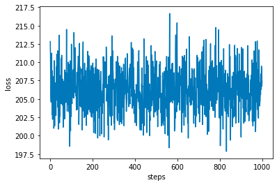
Hmm, not a lot of learning going on. Suspicious. Either something is wrong with the code (impossible!) or the model was initialized at the minimum loss.

Let’s take a look at some samples of the generative model.

z = p_z.sample((64,))
x_samples = Bernoulli(logits=nn(z)).sample() # (64, 784)
fig, axes = plt.subplots(8, 8, dpi=100)
for i, ax in enumerate(axes.flatten()):
  ax.imshow(1-x_samples[i].detach().cpu().reshape(28, 28), interpolation="none", cmap="gray")
  ax.axis("off")
plt.show()

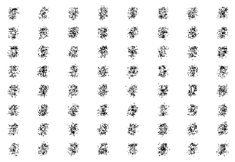
Hmm, these doesn’t really look like digits.

It’s also common to look at the averages that the generative model outputs, which often look better (and smoother), but these are not samples from the generative model. Be wary if you see very smooth samples, check that they are actual samples from the generative model and not an average. let’s take a look to see what’s going on.

p = t.sigmoid(nn(z)) # (64, 784)
fig, axes = plt.subplots(8, 8, dpi=100)
for i, ax in enumerate(axes.flatten()):
  ax.imshow(1-p[i].detach().cpu().reshape(28, 28), interpolation="none", cmap="gray")
  ax.axis("off")
plt.show()

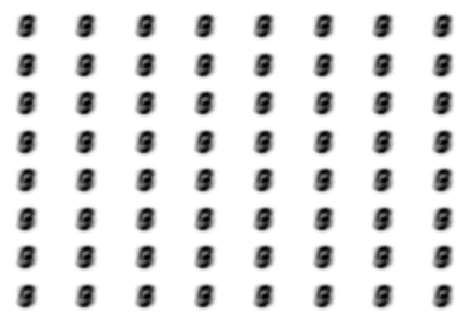
It appears the network has learned to output something like the average digit all the time. Let’s take a closer look at the loss to see if we can understand what’s going on. The loss is a lower bound to $\log p(x\theta)$. Can we derive what the missing term is, such that it’s an equality? This might help us to see what’s going on. We’ll add a term $D \geq 0$ to the RHS, and make the inequality an equality. This term $D \geq 0$ then represents what we need to add to the RHS to make the lower bound an equality.

\[\begin{align} \log p(x \vert \theta) &= \mathbb{E}_{z \sim p(z)} \log p(x \vert z, \theta) + D \\ D &= \log p(x \vert \theta) - \mathbb{E}_{z \sim p(z)} \log p(x \vert z, \theta) \\ &= \mathbb{E}_{z \sim p(z)} \log p(x \vert \theta) - \mathbb{E}_{z \sim p(z)} \log p(x \vert z,\theta) && \text{Since} \log p(x \vert \theta) \text{ doesn't depend on } z\\ &= \mathbb{E}_{z \sim p(z)} \left[ \log p(x \vert \theta) - \log p(x \vert z,\theta) \right] \\ &= \mathbb{E}_{z \sim p(z)} \left[ \log \frac{p(x \vert z, \theta)p(z)}{p(z \vert x, \theta)} - \log p(x \vert z,\theta) \right] && \text{Bayes rule}\\ &= \mathbb{E}_{z \sim p(z)} \left[ \log \frac{p(z)}{p(z \vert x, \theta)} \right] \\ &= D_{KL}\left[p(z) \vert \vert p(z \vert x,\theta)\right] \end{align}\]

The KL-Divergence is a positive measure of how different two distributions are, and its minimum is zero if and only if the two distributions are the same. It’s reassuring that the value we derived for $D$ is in fact greater than or equal to zero like we required it to be.

Inserting this definition of $D$ back we get,

\[\begin{align} \log p(x \vert \theta) &= \mathbb{E}_{z \sim p(z)} \log p(x \vert z, \theta) + D_{KL}\left[p(z) \vert \vert p(z \vert x,\theta)\right] \\ \log p(x \vert \theta) - D_{KL}\left[p(z) \vert \vert p(z \vert x,\theta)\right] &= \mathbb{E}_{z \sim p(z)} \log p(x \vert z, \theta) \end{align}\]

So now we can see what we’re actually maximizing. If we maximize the RHS, we’re either maximizing $\log p(x \vert \theta)$, which is what we want, or we’re minimizing the KL divergence between the prior $p(z)$ and the posterior $p(z \vert x, \theta)$. Let’s consider what doing the last thing means. The lowest the KL divergence can be is zero, when the two distributions are equal

\[D_{KL}(p(z) \vert \vert p(z \vert x, \theta)) = 0 \implies p(z) = p(z \vert x, \theta)\]

Which, by definition, implies that $z$ and $x$ are independent! So minimizing this KL term pushes $x$ and $z$ towards being independent. The only way $z$ and $x$ can be independent is if the network completely ignores $z$ and just outputs the same value for every $z$, which is in fact, exactly what seems to be happening!

We can also see that the RHS is not a consistent estimator of $\log p(x \vert \theta)$. The difference between the RHS, our estimator, and $\log p(x \vert \theta)$ does not approach zero as $N$, the amount of samples, approaches infinity. The difference is the KL term, which does not depend on the amount of samples $N$, rather it only depends on the parameters $\theta$.

In the next post we’ll use a better lower bound and finally get some MNIST digits!

Hosted on GitHub Pages — Theme by orderedlist