A meandering introduction to VAEs - part 2

The VAE is a so called Latent Variable Model (LVM). So what is a latent variable model? A simple latent variable model defines a probabilistic generative model of $x$ in the following way,

\[z \sim p(z \vert \theta)\] \[x \sim p(x \vert z, \theta) \,,\]

Which reads,

1. Draw a sample of the latent variables $z$ (conditioned on the model parameters $\theta$).
2. Draw a sample of $x$ conditioned on the drawn latent variables $z$ (and the the model parameters $\theta$).

The probability distribution over $x$ is then

\[p(x \vert \theta) = \int_z p(x, z \vert \theta) = \int_z p(x \vert z, \theta)p(z \vert \theta) \,.\]

For simplicity, authors rarely show the explicit conditioning on the model parameters $\theta$ in papers, or sometimes they’ll write $p_\theta(x)$, but it means the same thing.

So why might latent variable models be a good idea?

Manifold hypothesis. There’s a hypothesis that much of the data we’re interested in modelling can be described in fewer dimensions than what we observe. e.g. a low dimensional unobserved set of variables (objects and their properties, the position of the sun, etc.) and a complex process (physics / graphics) generates high dimensional observed data (images). Speech waveforms (high dim) are generated by the articulation of words (low dim), etc. If you just sample RGB pixel values randomly, it is extremely unlikely you get anything that looks like naturally observed images, so the “naturally observed” (hand wavy definition) images clearly occupies a very small part of the very large space of all possible RGB images.

Make better models. If we believe the manifold hypothesis, then the closer our models are to the true data generating process (physics, etc.) the better we can model the data.

Make simpler models. Pixels in natural images, cannnot be assumed to be independent, so you need to model the full joint distribution, but they might be approximately conditionally independent given the right latent variables (e.g. object positions, materials, classes, etc.), and these latent variables might themselves be approximately independent, allowing for easier modelling.

We hope to capture “interesting” and useful latent variables. For instance, gender, mood, hair style, age, etc. in face images. Or class (0-9) and style (slant, etc.) in handwritten digits. Capturing these latent factors of the data, might allow us to do better at downstream tasks, e.g. classifying images of digits, etc.

A latent variable model of MNIST digits

OK, so we have our probability distribution over $x$ for our LVM,

\[p(x \vert \theta) = \int_z p(x, z \vert \theta) = \int_z p(x \vert z, \theta)p(z \vert \theta) \,.\]

and if you recall, I said that maximizing the probability of the data under our model is all we need.

What does $p(z \vert \theta)$ and $p(x \vert z, \theta)$ actually look like though? And how do we evaluate the integral? At this point an example is instructive. We’ll define a LVM on MNIST, and get back to the integral.

MNIST is arguably the “hello world” dataset of generative modelling. It consists of $70.000$ $28 \times 28$ grayscale images of handwritten digits (and associated labels 0-9). Here are some examples.

The values of each pixel in the original dataset is between 0 and 1, and can be seen as an intensity. We’ll use a version called static MNIST where the pixels have instead been sampled with probability equal to these intensities, such that they are binary, 0 or 1, since this is the norm in the generative modelling litterature. For simplicity we’ll flatten each $28 \times 28$ image into a vector of $784$ binary values, such that $x_j$ denotes the $j$’th value.

Now, let’s specify our model in a little more detail,

\[z_i \sim \mathcal{N}(z_i \vert \mu=0, \sigma=1) \, \text{for} \, i \, \text{in} \, [1, ..., K]\,,\] \[[p_1, ..., p_{784}] = \text{NN}_\theta([z_1, ..., z_k]) \,,\] \[x_j \sim \text{Bernoulli}(x_j \vert p = p_j) \, \text{for} \, j \, \text{in} \, [1, ..., 784] \,.\]

This reads,

1. Sample $K$ latent variables from independent normal distributions with mean 0 and standard deviation 1. K is a hyper-parameter, the size of our latent space, something we’ll decide on later.
2. Turn those $K$ latent variables into a vector of length $K$ and pass that vector through a Neural Network with $\theta$ parameters, the weights and biases of the network. The output of the neural network is a vector of $784$ probabilities (0-1). Notice that we’re using an equal sign here, and not a $\sim$ sign, since it’s a deterministic computation not a sample.
3. Sample the 784 $x_j$ values from independent Bernoulli distributions with those 784 probabilities.

That is our generative model. Following the recipe above we can now generate binary vectors with length 784. Will they look like MNIST digits, if reshaped back into $28 \times 28$? That depends entirely on the parameters $\theta$. We’re relying on the neural networks extreme flexibility to turn a $K$ dimensional normal distribution into a $784$ dimensional bernoulli distribution that looks like handwritten digits. I think it’s instructive to actually implement our generative model at this point, and look at some samples.

I’ll use $K=2$, a relatively simple neural network of a single hidden layer with 128 hidden units, ELU non-linearities and a Sigmoid non-linearity for the last layer to map to (0-1), and I’ll use pytorch.distributions for all the probability distributions.

import torch as t
import matplotlib.pyplot as plt
from torch.distributions import Normal, Bernoulli

K = 2
n_hid = 128

nn = t.nn.Sequential(
    t.nn.Linear(2, n_hid), t.nn.ELU(),
    t.nn.Linear(n_hid, n_hid), t.nn.ELU(),
    t.nn.Linear(n_hid, 784), t.nn.Sigmoid()
)

print("model parameters:")
for name, param in nn.named_parameters():
  print("name: %s \t shape: %s"%(name, param.shape))


print("samples:")
with t.no_grad():
  z = Normal(loc=t.zeros(K), scale=t.ones(K)).sample((10,)) # step 1. z ~ p(z). shape: (10, 2)
  p = nn(z) #Step 2. shape: (10, 784)
  x = Bernoulli(probs=p).sample() #Step 3. x ~ p(x  \vert  z, 𝜃). shape: (10, 784) 

fig, axes = plt.subplots(1, 10, dpi=100)
for ax, x_sample in zip(axes, x):
  ax.imshow(1-x_sample.reshape(28, 28), origin="lower left", interpolation="none", cmap="gray")
  ax.axis("off")
plt.show()

model parameters:
name: 0.weight 	 shape: torch.Size([128, 2])
name: 0.bias 	 shape: torch.Size([128])
name: 2.weight 	 shape: torch.Size([128, 128])
name: 2.bias 	 shape: torch.Size([128])
name: 4.weight 	 shape: torch.Size([784, 128])
name: 4.bias 	 shape: torch.Size([784])
samples:

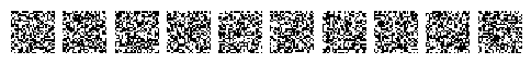
That certainly doesn’t look like handwritten digits, which is no surprise since all our parameters $\theta$ are just initialized randomly.

Please make sure you understand the code above before moving on. Notice how closely it resembles the model definition; the model definition is quite literally a recipe for sampling from the model. Note: I’m showing $1-x$ so that the “on” pixels are dark, and the “off” pixels are light, since it looks better on a white background. It’s purely an aesthetic detail.

So how do we find $\theta$? As before, by maximizing the probability of the observed data under our model. Again, this is equivialent to maximizing the log probability of the observed data under the model.

\[\begin{align} \theta_{MLE} &= \max_\theta p(x \vert \theta) \\ &= \max_\theta \log p(x \vert \theta) \\ &= \max_\theta \log \int_z p(x \vert z, \theta)p(z) \,. \end{align}\]

Note: I removed the dependence on $\theta$ in the prior, because our prior $p(z)$ does not have any parameters.

Just to be very clear what I mean, I’ll write out the full definition of $p(x \vert \theta)$ for our model,

\[p(x \vert \theta) = \int_z p(x \vert z, \theta)p(z) = \int_{z_1} ... \int_{z_K} \prod_{j=1}^{784} \text{Bernoulli}(x_j \vert p=p_j) \prod_{i=1}^K \mathcal{N}(z_i \vert \mu=0, \sigma=1) \,,\]

where $p_j$ are the output of the neural network.

We’ll continue with the simple form however, to keep things somewhat neat.

Computing $p(x \vert \theta)$ or $\log p(x \vert \theta)$

So it all boils down to computing $p(x \vert \theta)$ or $\log p(x \vert \theta)$, so we can maximize it. How to do this, precisely and efficiently is really one of the core questions of latent variable models. A plethora of methods have been proposed, and it’s instructive to go through some of them before getting to how VAEs approach it. I’ll try to proceed in the order of simplest first, and show how and when those approaches come up short, which will motivate the more advanced approaches.

Approach 1 - Estimate $p(x \vert \theta)$ with samples

First we’ll note that by definition of the expectation, $p(x \vert \theta)$ is equal to the expectation over $p(x \vert z, \theta)$ with $z$ drawn from $p(z)$,

\[p(x \vert \theta) = \int_z p(x \vert z, \theta)p(z) = \mathbb{E}_{z \sim p(z)} p(x \vert z, \theta) \,.\]

We can write the expectation as an average over an infinite amount of samples from $p(z)$,

\[p(x \vert \theta) = \mathbb{E}_{z \sim p(z)} p(x \vert z, \theta) = \lim_{N \rightarrow \infty } \frac{1}{N} \sum_{i=1}^N p(x \vert z_i \sim p(z), \theta) \,.\]

Unfortunately, we can’t sample an infinite amount of samples, so we’ll have to sample a finite amount, which means we’ll be approximating this expectation

\[p(x \vert \theta) = \mathbb{E}_{z \sim p(z)} p(x \vert z, \theta) \approx \frac{1}{N} \sum_{i=1}^N p(x \vert z_i \sim p(z), \theta) \,.\]

where $N$, the amount of samples, is a hyper-parameter we’ll have to choose. This is an unbiased and consistent estimator, meaning it doesn’t systematically under or over-estimates the true expectation, and it converges to the true expectation in the limit of infinite samples, which is great!

There’s just one snag, the probabilities tend to underflow. Let’s assume our NN is pretty good and outputs $p=0.8$ for all the pixels that are $1$, and $p=0.2$ for all the pixels that are $0$, then $p(x \vert z, \theta) = \prod_{i=1}^{784} p_j^{x_j}(1-p_j)^{1-x_j} = 0.8^{784}$, which is a small number, but definitely not 0, but when we ask the computer to evaluate it, it underflows, and say it’s 0.

import torch as t

print(t.tensor([0.8], dtype=t.float32)**784)

tensor([0.])

In general, computing directly with probabilities quickly becomes very unstable, so for now on we’ll turn our attention to computing $\log p(x \vert \theta)$ in the next part.

Hosted on GitHub Pages — Theme by orderedlist