A meandering introduction to VAEs - part 1

In this series of posts I’ll work my way up to explaining how the Variational Autoencoder (VAE) works, starting from almost scratch. The VAE is an extremely popular probabilistic generative model, which led to great advances in generative modelling. I’ll try to explain it as gently as possible, with a focus on why and the background behind the steps, since the VAE was not invented in a vacuum. Ideally, as you are reading this, every step should feel logical, if not please let me know.

Unfortunately I cannot explain everything, so I have to draw the line somewhere. In order to understand this note, you’ll need to have a basic understanding of probability, neural networks and gradient descent. Make sure you understand the following points

1. \(p(a,b) = p(a \vert b)p(b) = p(b \vert a)p(a)\)
2. $p(a) = \int_b p(a,b)$
3. Bayes rule: $p(a \vert b) = \frac{p(b \vert a)p(a)}{p(b)}$
4. Neural networks are very flexible parameterized functions and they can be trained to approximate functions with optimization techniques like gradient descent.

Probabilistic Modelling Preliminaries

The VAE is a probabilistic generative model. Probabilistic modelling aims to model data in terms of probability distributions, and is one of the main paradigms of unsupervised learning. So what does a very simple probabilistic model of data looks like?

Let’s assume we want to model the weight of newborns. We’ll describe our model by defining the generative process. That is, the process by which our model generates data. In the case of the weight of newborns, $x$, we’ll write it as

\[x \sim \mathcal{N}(x \vert \mu, \sigma) \,,\]

which means: “$x$ is distributed according to a normal distribution with mean $\mu$ and standard deviation $\sigma$”. You can also read it as a recipe for generating data, in which case it reads: “sample $x$ from a normal distribution with mean $\mu$ and standard deviation $\sigma$”. Writing down the generative process like this is the standard notation for probabilistic models. Note that this model is probably not a perfect model since it can lead to negative weights, which we know is impossible, but for now it’s fine. The $\mu$ and $\sigma$ are unspecified for now and are the parameters of our model. It’s common to denote all the parameters of the model by $\theta$, so that in this case $\theta = {\mu, \sigma}$.

Now, let’s assume we observe the following weights (in grams) $\mathbf{x}=[x_1, x_2, x_3]=[2642, 3500, 4358]$, such that $x_1 = 2642$, $x_2=3500$ and $x_3 = 4358$, and this is all the data we observe. What should our model parameters be then, such that we have the best possible model of the observed data?

The parameters that corresponds to the best possible model of the observed data is known as the maximum likelihood estimate (MLE). They are the parameters that maximize the probability of the observed data under the model.

\[\theta_{MLE} = \max_\theta p(x \vert \theta)\]

This corresponds to finding the model which is the most likely to have generated the observed data. For numerical reasons it’s often better to maximize the log-probability, and since log is a monotonic function it preserves the location of the maximum,

\[\theta_{MLE} = \max_\theta p(x \vert \theta) = \max_\theta \log p(x \vert \theta) \,.\]

When we defined the model we implicitly defined the data to be independent and identically distributed (IID), since each sample $x_i$ did not depend on the other samples $x_j$. As such, the joint probability of the observed data is

\[p(\mathbf{x} \vert \theta) = p(x_1 \vert \theta)p(x_2 \vert \theta)p(x_3 \vert \theta) = \prod_{i=1}^3 \mathcal{N}(x_i \vert \mu, \sigma) \,,\]

and

\[\log p(\mathbf{x} \vert \theta) = \sum_{i=1}^3 \log \mathcal{N}(x_i \vert \mu, \sigma) \,,\]

Let’s take a look at what the log probability of the observed data looks like for different values of $\mu$ and $\sigma$.

import numpy as np
from scipy.stats import norm
import matplotlib.pyplot as plt

x = np.array([2642, 3500, 4358])

N = 100
means = np.linspace(3000, 4000, N)
stds = np.linspace(500, 1600, N)
logpdfs = np.zeros((N, N))
for i, mean in enumerate(means):
  for j, std in enumerate(stds):
    logpdfs[i, j] = norm.logpdf(x, loc=mean, scale=std).sum()

plt.figure(figsize=(8,8))
plt.imshow(logpdfs.T, origin="lower left", interpolation='none', extent=[means.min(), means.max(), stds.min(), stds.max()])
plt.plot(x.mean(), x.std(), 'rx')
plt.xlabel("mean")
plt.ylabel("std")
plt.title("log p(x = [2642, 3500, 4358]  \vert  mean, std)")
plt.colorbar()
plt.show()

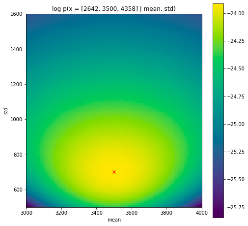
As you can see the log probability of the observed data has a peak at the expected maximum likelihood estimate which is the empirical mean and standard deviation. However, the peak is quite flat; there’s many values of $\mu$ and $\sigma$ that are almost as good models of the data. If we were good Bayesians we should recognize that 1) we have prior information on these parameters and 2) that we are uncertain about these parameters, even after seeing data. But that is for another post. Today we’re happy with just picking the set of parameters that result in the best model of the data, the maximum likelihood estimate. Note that in this case, the MLE had a simple analytical solution, but we could also have found it using optimization techniques such as gradient ascent. This is often the approach taken in more complex models.

One thing remains, which is to show that this is a generative model; we can sample new data from it.

norm.rvs(loc=x.mean(), scale=x.std(), size=10)

array([3741.7468832 , 2879.43346711, 2889.47198528, 3431.85622032,
       3118.47621065, 2597.82799007, 3244.1547452 , 4279.39183118,
       3058.90122162, 3175.86724978])

Does this look like the real data? Yea, it looks pretty good I think. Those all seem like sensible weights for newborns. I don’t think I could tell these apart from actual weights (if they were rounded to whole grams).

To summarize, to create a probabilistic generative model we define parameterized probabilistic models, and find the parameters that maximize the log probability of the observed data under the model.

If you’re not feeling completely confident about this, here’s a little exercise you can do.

Over three days you look at a ride-sharing app at random times of the day and find the following number of cars within a short distance of your home address $\mathbf{x} = [3, 4, 1]$.

1. Define a simple probabilistic model of how data like this could be generated. Write it down in standard notation. (hint: it’s not a normal distribution, since those are integers, not real numbers)
2. What are the model parameter(s)?
3. What is the MLE of the parameter(s)?
4. What is $\log p(\mathbf{x} \vert \theta_{MLE})$?

Hosted on GitHub Pages — Theme by orderedlist